How It Works¶

Technical deep-dive into DeepAugment’s design and methodology.

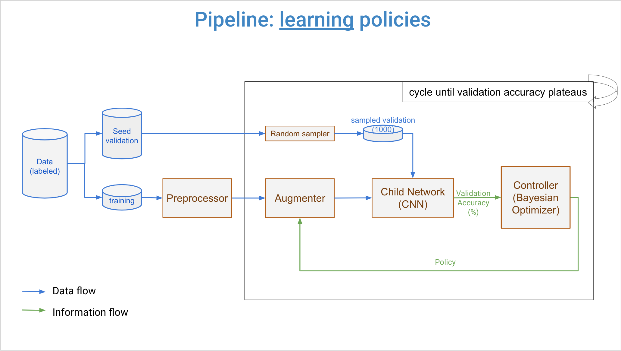
Overview¶

DeepAugment automates the search for optimal image augmentation policies using Bayesian Optimization. It consists of three main components that work together in an iterative loop:

Controller: Samples augmentation policies using Bayesian Optimization
Augmenter: Transforms images according to policies
Child Model: Evaluates policy quality through training

The Optimization Loop¶

The core workflow:

Controller samples a new augmentation policy
Augmenter applies the policy to training images
Child model trains on augmented images
Validation accuracy is computed (reward)
Controller updates with (policy, reward) pair
Repeat until convergence or max iterations

This process discovers which augmentation combinations work best for your specific dataset.

Why Bayesian Optimization?¶

Comparison of Hyperparameter Optimization Methods¶

Method	Iterations Needed	Computation Cost	Accuracy	Complexity
Grid Search	Very High	Very High	Medium	Low
Random Search	High	High	Medium	Low
Bayesian Optimization	Low (~100-300)	Low	High	Medium
Reinforcement Learning	Very High (~15,000)	Very High	High	High

AutoAugment vs DeepAugment¶

Google’s AutoAugment uses Reinforcement Learning:

Iterations needed: ~15,000
Time: Days to weeks
Cost: Requires massive computational resources
Accessibility: Not practical for most users

DeepAugment uses Bayesian Optimization:

Iterations needed: ~100-300
Time: Hours
Cost: ~$13 on AWS for CIFAR-10
Accessibility: Practical for individual researchers and small teams

Performance: Bayesian Optimization achieves comparable or better results with ~100x fewer iterations.

Bayesian Optimization Details¶

How It Works¶

Bayesian Optimization maintains a surrogate model that predicts the quality of unexplored policies:

Build surrogate model from previous evaluations
Acquisition function identifies promising policies to try next
Evaluate the selected policy
Update surrogate model with new result
Repeat

DeepAugment uses:

Surrogate: Random Forest Estimator
Acquisition: Expected Improvement (EI)
Library: scikit-optimize

Expected Improvement¶

The acquisition function balances:

Exploitation: Try policies similar to current best
Exploration: Try unexplored regions of policy space

This balance is key to efficient optimization.

Mathematical Formulation¶

The optimization problem:

\[\begin{split}\\mathbf{p}^* = \\arg\\max_{\\mathbf{p} \\in \\mathcal{P}} f(\\mathbf{p})\end{split}\]

Where:

$\\mathbf{p}$ is an augmentation policy
$\\mathcal{P}$ is the space of all possible policies
$f(\\mathbf{p})$ is the validation accuracy with policy $\\mathbf{p}$
$\\mathbf{p}^*$ is the optimal policy

The challenge: $f(\\mathbf{p})$ is expensive to evaluate (requires training a model).

Bayesian Optimization efficiently explores $\\mathcal{P}$ by building a probabilistic model of $f$.

Policy Representation¶

Policy Structure¶

A policy consists of $N$ operations (default $N=4$):

\[\begin{split}\\mathbf{p} = [(t_1, m_1), (t_2, m_2), ..., (t_N, m_N)]\end{split}\]

Where:

$t_i$ is a transform type (categorical: 1 to 26)
$m_i$ is magnitude (continuous: 0.0 to 1.0)

Example policy:

[
    ('rotate', 0.8),      # t₁=rotate, m₁=0.8
    ('brightness', 0.5),  # t₂=brightness, m₂=0.5
    ('blur', 0.3),        # t₃=blur, m₃=0.3
    ('flip_h', 0.9),      # t₄=flip_h, m₄=0.9
]

Search Space Size¶

For $N=4$ operations with 26 transforms:

Categorical dimensions: 26 choices × 4 = $26^4 = 456,976$ combinations
Continuous dimensions: $[0, 1]^4$ (infinite)
Total: Extremely large search space

This is why naive grid search is infeasible and Bayesian Optimization is necessary.

Transform Library¶

DeepAugment includes 26 modern transforms from torchvision v2:

Geometric Transforms (8)¶

rotate: Rotation by angle
flip_h: Horizontal flip
flip_v: Vertical flip
affine: Affine transformation
shear: Shear transformation
perspective: Perspective transformation
elastic: Elastic deformation
random_crop: Random cropping

Color Transforms (5)¶

brightness: Brightness adjustment
contrast: Contrast adjustment
saturation: Saturation adjustment
hue: Hue adjustment
color_jitter: Combined color jittering

Advanced Color (7)¶

sharpen: Sharpening
autocontrast: Auto contrast
equalize: Histogram equalization
invert: Color inversion
solarize: Solarization
posterize: Posterization
grayscale: Grayscale conversion

Blur & Noise (2)¶

blur: Gaussian blur
gaussian_noise: Additive Gaussian noise

Occlusion (2)¶

erasing: Random erasing
cutout: Cutout augmentation

Advanced (2)¶

channel_permute: Channel permutation
photometric_distort: Photometric distortion

Each transform’s magnitude is normalized to [0, 1] for uniform optimization.

Child Model¶

Architecture¶

The child model is a lightweight CNN designed for fast training:

Parameters: 1,250,858 (for 32×32 images)
Training time: ~30 seconds per iteration on V100 GPU
Architecture: 3 convolutional blocks + fully connected layers

Design Principles¶

The child model is intentionally small:

Fast evaluation: Each policy needs training from scratch
Good proxy: Performance correlates with larger models
Memory efficient: Fits in GPU memory with large batches

Key insight: Small model + good augmentation ≈ Large model + weak augmentation

Custom Models¶

You can use your own model as the child model:

aug = DeepAugment(
    X_train, y_train, X_val, y_val,
    model=MyCustomModel
)

Trade-off: Larger models give more accurate policy evaluation but take longer.

Reward Function¶

Default Reward¶

The reward is the validation accuracy of the child model trained with the policy:

\[\begin{split}r(\\mathbf{p}) = \\text{Accuracy}_{\\text{val}}(\\text{Model trained with } \\mathbf{p})\end{split}\]

Implementation details:

Model trained for $E$ epochs (default $E=10$)
Reward is mean of top $K$ validation accuracies (default $K=3$)
This reduces noise from training variance

Custom Rewards¶

You can define custom reward functions:

def my_reward(entry):
    score = entry['score']
    policy = entry['policy']

    # Example: Penalize complex policies
    complexity = len(policy)
    return score - 0.01 * complexity

aug = DeepAugment(
    X_train, y_train, X_val, y_val,
    custom_reward_fn=my_reward
)

This allows optimizing for multiple objectives (accuracy + simplicity, speed, etc.).

Data Pipeline¶

Training Data Flow¶

Validation Data Flow¶

Key Points¶

Augmentation applied per-epoch: Same image gets different augmentations each epoch
Validation not augmented: Ensures unbiased evaluation
Random sampling: Magnitude determines probability/intensity of each transform
Sequential application: Transforms applied in policy order

Design Principles¶

DeepAugment follows several design philosophies:

Convention over Configuration¶

Sensible defaults for everything:

# This works out of the box
best = optimize(X, y, iterations=50)

Rails Doctrine¶

Optimize for programmer happiness: Clean API, readable code
Convention over configuration: Defaults work well
Progress over stability: Use modern approaches
Omakase: Curated, opinionated stack

Single Source of Truth¶

Each piece of logic lives in exactly one place:

Policy representation → policy.py
Transforms → transforms.py
Training → trainer.py
Search → search.py

This makes the codebase maintainable and extensible.

Academic Foundation¶

DeepAugment builds on strong theoretical foundations:

Key Papers¶

AutoAugment (Cubuk et al., 2018): Original idea of learned augmentation
Bayesian Optimization Review (Shahriari et al., 2016): BO theory
Neural Architecture Search (Zoph et al., 2016): Search methodology
Cutout (DeVries & Taylor, 2017): Occlusion augmentation

Novel Contributions¶

DeepAugment’s contributions:

First application of Bayesian Optimization to augmentation policy search
Minimized child model for computational efficiency
Practical implementation accessible to individual researchers
Open source with complete code and documentation

Performance Validation¶

Validated on CIFAR-10 with WRN-28-10:

Baseline: 91.5% accuracy
With DeepAugment: 95.0% accuracy
Improvement: 8.5% absolute (60% error reduction)

See Citation & References for how to cite this work.

Computational Complexity¶

Time Complexity¶

For $T$ iterations, $E$ epochs, $N$ samples, batch size $B$:

\[\begin{split}\\text{Time} \\approx T \\times E \\times \\frac{N}{B} \\times t_{\\text{forward+backward}}\end{split}\]

For CIFAR-10 with default settings:

$T=100$ iterations
$E=10$ epochs
$N=2000$ samples
$B=64$ batch size
:math:`t=0.01`s per batch on V100

Total time: ~4.2 hours (~$13 on AWS p3.x2large)

Space Complexity¶

Memory usage:

Model parameters: ~1.2M × 4 bytes = 5 MB
Batch storage: batch_size × image_size × 4 bytes
Optimizer state: 2× model size = 10 MB

Total: ~100-200 MB on GPU (very efficient)

How It Works¶

Overview¶

The Optimization Loop¶

Why Bayesian Optimization?¶

Comparison of Hyperparameter Optimization Methods¶

AutoAugment vs DeepAugment¶

Bayesian Optimization Details¶

How It Works¶

Expected Improvement¶

Mathematical Formulation¶

Policy Representation¶

Policy Structure¶

Search Space Size¶

Transform Library¶

Geometric Transforms (8)¶

Color Transforms (5)¶

Advanced Color (7)¶

Blur & Noise (2)¶

Occlusion (2)¶

Advanced (2)¶

Child Model¶

Architecture¶

Design Principles¶

Custom Models¶

Reward Function¶

Default Reward¶

Custom Rewards¶

Data Pipeline¶

Training Data Flow¶

Validation Data Flow¶

Key Points¶

Design Principles¶

Convention over Configuration¶

Rails Doctrine¶

Single Source of Truth¶

Academic Foundation¶

Key Papers¶

Novel Contributions¶

Performance Validation¶

Computational Complexity¶

Time Complexity¶

Space Complexity¶

See Also¶

References¶